INTRODUCTION TO MATLAB

Chapter 3
Input, Calculating, and Output

3.1 Input
To have a script request and assign a value to the variable N from the keyboard use
N=input(' Enter a value for N - ')

If you enter a single number, like 2.7, then N will be a scalar variable. If you enter an
array, like this: [1,2,3,4,5], then N will be an array. If you enter a matrix, like this:
[1,2,3;4,5,6,7,8,9], then N will be a 3x3 matrix. And if you don't want the variable you
have entered to echo on the screen, end the input command line with a semicolon.

You can also enter data from a le filled with rows and columns of numbers. Matlab
reads the le as if it were a matrix with the first line of the le going into the first row of
the matrix. If the le were called data.fil and looked like this
1 2 3
4 5 6
7 8 9

then the Matlab command
load data.fil

would produce a matrix called data filled with the contents of the le.

3.2 Calculating
Matlab only crunches numbers. It doesn't do any symbolic algebra, so it is much less
capable than Mathematica or Maple. But because it doesn't have to do hard symbolic
stuff, it can handle numbers much faster than Mathematica or Maple can. (Testimonial:
"I, Scott Bergeson, do hereby certify that I wrote a data analysis code in Maple that took
25 minutes to run. When I converted the code to Matlab it took 15 seconds.") Here's a
brief summary of what it can do with numbers, arrays, and matrices.

3.3 Add and Subtract
Matlab knows how to add and subtract numbers, arrays, and matrices. As long as A and
B are two variables of the same size (e.g., both 2 3 matrices), then A + B and A - B will
add and subtract them as matrices:
A=[1,2,3;4,5,6;7,8,9]
B=[3,2,1;6,4,5;8,7,9]
A+B
A-B

3.4 Multiplication
The usual multiplication sign * has special meaning in Matlab. Because everything in
Matlab is a matrix, * means matrix multiply. So if A is a 3 × 3 matrix and B is another
3 × 3 matrix, then A * B will be their 3 × 3 product. Similarly, if A is a 3 × 3 matrix and C
is a 3 × 1 matrix (column vector) then A * C will be a new 3 × 1 column vector. And if you
want to raise A to a power by multiplying it by itself n times, you just use
A^n

For a language that thinks everything in the world is a matrix, this is perfectly natural.
Try
A*B
A*[1,2,3]
A^3

But there are lots of times when we don't want to do matrix multiplication. Sometimes
we want to take two big arrays of numbers and multiply their corresponding elements
together, producing another big array of numbers. Because we do this so often (you will
see many examples later on) Matlab has a special symbol for this kind of multiplication:
.*

For instance, the dot multiplication between the arrays [a,b,c] and [d,e,f] would be the
array [a*d,b*e,c*f]. And since we might also want to divide two big arrays this way, or
raise each element to a power, Matlab also allows the operations
./
.^

For example, try
[1,2,3].*[3,2,1]
[1,2,3]./[3,2,1]
[1,2,3].^2

These "dot" operators are very useful in plotting functions and other kinds of signal processing.
( You are probably confused about this dot business right now. Be patient. When
we start plotting and doing real calculations this will all become clear.)

3.5 Arithmetic with Array Elements
If you just want to do some arithmetic with specific values stored in your arrays, you can
just access the individual elements. For instance, if you want to divide the third element of
A by the second element of B, you would just use
A(3)/B(2)

Note that in this case the things we are dividing are scalars (or 1 × 1 arrays in Matlab's
mind), so Matlab will just treat this like the normal division of two numbers (i.e. we don't
have to use the ./ command, although it wouldn't hurt if we did).

3.6 Complex Arithmetic
Matlab works as easily with complex numbers as with real ones. The variable i is the usual
imaginary number unless you are so foolish as to assign it some other value, like
this:
i=3

If you do this you no longer have access to imaginary numbers, so don't ever do it. If you
accidentally do it the command clear i will restore it to its imaginary luster. By using i
you can do complex arithmetic, like this
z1=1+2i
% or you can multiply by i, like this
z1=1+2*i

z2=2-3i
% add and subtract
z1+z2
z1-z2
% multiply and divide
z1*z2
z1/z2

And like everything else in Matlab, complex numbers work as elements of arrays and matrices
as well.

When working with complex numbers we quite often want to pick o the real part or
the imaginary part of the number, find its complex conjugate, or find its magnitude. Or
perhaps we need to know the angle between the real axis and the complex number in the
complex plane. Matlab knows how do all of these
z=3+4i
real(z)
imag(z)
conj(z)
abs(z)
angle(z)

Matlab also knows how to evaluate many of the functions discussed in the next section
with a complex argument. Perhaps you recall Euler's famous formula
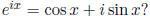
Matlab knows it too.
exp(i*pi/4)

Matlab knows how to handle complex arguments for all of the trig, exponential, and hyperbolic
functions. It can do Bessel functions of complex arguments too.

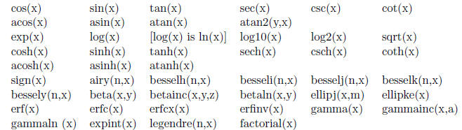
3.7 Mathematical Functions
Matlab knows all of the standard functions found on scientific calculators and even many
of the special functions like Bessel functions. We will give you a list below of a bunch of
them, but first you need to know an important feature that they all share. They work just
like the "dot" operators discussed in the previous section. This means, for example, that it
makes sense to take the sine of an array: the answer is just an array of sine values, e.g.,
sin([pi/4,pi/2,pi])= [0.7071 1.0000 0.0000]

OK, here's the list of function names that Matlab knows about. You can use online
help to find details about how to use them. Notice that the natural log function ln x is the
Matlab function log(x).

3.8 Housekeeping Functions
Here are some functions that don't really do math but are useful in programming.

abs(x) the absolute value of a number (real or complex)
clc clears the command window, useful for beautifying printed output
ceil(x) the nearest integer greater than x
clear clears all assigned variables
close all closes all figure windows
close 3 closes figure window 3
fix(x) the nearest integer to x looking toward zero
iplr(A) flip a matrix A, left for right
ipud(A) flip a matrix A, up for down
oor(x) the nearest integer less than x
length(a) the number of elements in a vector
mod(x,y) the integer remainder of x/y, see online help if x or y are negative
rem(x,y) the integer remainder of x/y, see online help if x or y are negative
rot90(A) rotate a matrix A by 90°
round(x) the nearest integer to x
sign(x) the sign of x and returns 0 if x=0
size(c) the dimensions of a matrix

Try floor([1.5,2.7,-1.5]) to see that these functions operate on arrays and not just
on single numbers.

3.9 Output
Now hold on for a second, so far you may have executed most of the example Matlab
commands in the command window. From now on it will prepare you better for the more
difficult material coming up if you have both a command window and an M- le window
open. Put the examples to be run in the M- le (call it junk.m), then execute the examples
from the command window by typing
junk

OK, let's learn about output. To display printed results you can use the fprintf command.
For full information type
help fprintf

but to get you started, here are some examples. Try them so you know what each one
produces. (Here's a hint: the stuff inside the single quotes is a string which will print on
the screen, % is where the number you are printing goes, and the stuff after % is a format
code. A g means use \whatever" format, if the number is really big or really small, use
scientific notation, otherwise just throw 6 significant figures on the screen in a format that
looks good. The format 6.2f means use 2 decimal places and fixed-point display with 6
spaces for the number. An e means scientific notation, with the number of decimal places
controlled like this: 1.10e.)
fprintf(' N =%g \n',500)
fprintf(' x =%1.12g \n',pi)
fprintf(' x =%1.10e \n',pi)
fprintf(' x =%6.2f \n',pi)
fprintf(' x =%12.8f y =%12.8f \n',5,exp(5))

Note:\n is the command for a new line. If you want all the details on this stuff , look in a
C-manual or Chapter 10 of Mastering Matlab 6.

This command will also write output to a le. Here is an example from online help that
writes a le filled with a table of values of x and exp(x) from 0 to 1. Note that when using
Windows that a different line-feed character must be used with \r \n replacing \n (see the
fprintf below.)

Note: the example in the box below is available on the Physics 330 course website, as
are all of the examples labeled in this way in this booklet.

After you try this, open file1.txt, look at the way the numbers appear in it, and compare
them to the format commands %6.2f and %12.8f to learn what they mean. Write the file
again using the %g format for both columns and look in the file again.