Vector operations on TI Calculators

TI-89 SCALAR (DOT) PRODUCT OF VECTORS

keystrokes:

<2^nd> then <5>MATH then nd <4> to select MATRIX from menu
scroll down menu to item L:Vector ops then press <ENTER>
scroll down menu to item 3:DotP( then press <ENTER>
In the command line enter, for example: [1,2,3],[4,5,6]) then press <ENTER>
note that the opening “(“ was already displayed
result display will be 32, which is the dot product of (1i + 2j + 3k) & (4i + 5j + 6k)

TI-89 VECTOR (CROSS) PRODUCT OF VECTORS

keystrokes:
<2^nd> then <5>MATH then <4> to select MATRIX from menu
scroll down menu to item L:Vector ops then press <ENTER>
scroll down menu to item 2:CrossP( then press <ENTER>
In the command line enter, for example: [1,2,3],[4,5,6]) then press <ENTER>
note that the opening “(“ was already displayed
resulting display will be [-3, 6, -3] which represents -3i + 6j - 3k,
the cross product of (1i + 2j + 3k) × (4i + 5j + 6k)

Solving Simultaneous Equations With TI-82, TI-83, TI-83 Plus, and TI-83 Plus
Silver Edition Graphing Calculators
(courtesy of Mr. Nabil Thalji)

Simultaneous equations can be solved quickly with several TI series graphing calculators
using augmented matrices.

Procedure:
1. Press [2nd][x^-1] to access the matrix menu (for TI-82 and regular TI-83, this is an
actual key and not the second function of the [x^-1] key).
2. Hit the right arrow button twice to scroll over to the EDIT tab, and select the
matrix you want to edit (it does not matter which one you choose).
3. To edit the matrix, first enter the dimensions of the matrix. The dimensions
should be as follows: If you have two simultaneous equations, the dimensions
should be 2x3. If you have three equations, it should be 3x4. For 4, 4x5, and so
on.
4. Now begin entering the values into the matrix. Use one row per equation. Use
ONE column for each variable. The following is an example of how to enter the
values into the matrix properly:

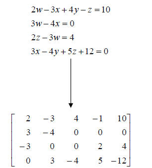
Note that all the w coefficients are in the same column, and all the x coefficients are in
the same column and so forth. Note that all constants are in the LAST column. Also note
that each equation must be rewritten to the form Aw+Bx+Cy+Dz=C in order to be
translated directly into the matrix.

5. Hit [2nd][MODE], which is the QUIT function. This gets you out of the matrix
editor. Hit [2nd][x-1] to return to the matrix menu and hit the right arrow key once to
get to the MATH menu. Scroll down until you get to the function “rref(” (which is the
12^th function in the list), and hit enter. Then return to the matrix menu again ([2nd][x-
1]), find the matrix you created (under the NAMES tab), and hit enter to select it. This
puts the matrix within the rref( function so you should see something like this:
“rref([A]”. Hit enter again and you will get a reduced matrix that looks something
like this:

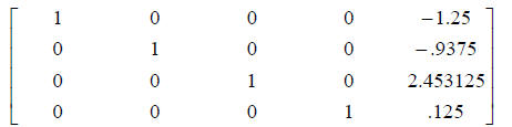
(Note: the matrix may be too large to fit completely on the screen, so use the right and
left arrow buttons to see the entire matrix. The above matrix is the solution of the
example described in step 4.)

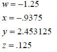
6. Recall which column represented which variable in your initial augmented matrix.
The matrix in step 5 represents the following:

This method is very rapid once you have done it once or twice, and doesn’t require
multiple matrices like Cramer’s rule. It is based on the reduction of an augmented matrix
(shown in step 4) into what’s known as reduced row echelon form (shown in step 5).
Augmented matrices are terrible to reduce if you have to do it by hand, but incredibly
simple if done on a calculator.