Solution of Simultaneous Linear Equations

•matrix representation of a system of simultaneous linear
equations

–Ax=b

•most common in physics: “square systems”

•linear independence of equations

–The determinant det(A) give you a measure of closeness to singularity

It is also possible to expand a determinant along a row or column using Laplace's formula ,which is efficient
for relatively small matrices .To do this along row i ,say ,we write

where the represent the matrix cofactors ,i.e. is times the minor,which is the
determinant of the matrix that result from A by removing the i-th row column.

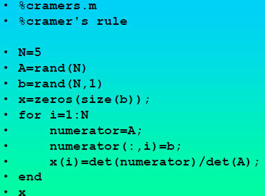
•Cramer’s Rule

Elementary formulation

The system of equations is represented in matrix multiplication form as:

where the square matrix A is invertible and the vector x is the column vector of the variables:
The theorem then states that:

where is the matrix formed by replacing the ith column of A by the column vector c

•Computationally, Cramer’s Rule is generally inefficient and thus
not used in practical applications which may involve many
equations. However, it is of theoretical importance in that it gives
an explicit expression for the solution of the system.

•We can make a script that implements Cramer’s rule

•We can make Cramer’s rule into a function

–x=cramers(A,b)

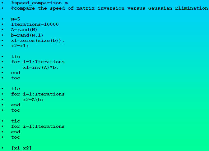
MATLAB gives you other ways to solve Ax=b

–matrix inversion:

–in MATLAB: x=inv(A)*b

•The best way to solve Ax=bin MATLAB is x=A\b

–Uses Gaussian elimination
–somewhat faster than matrix inversion

•we can compare speeds in a little code

–warning message if nearly singular
–error message if singular

–what happens for an underdetermined system?
–what happens for an overdetermined system?

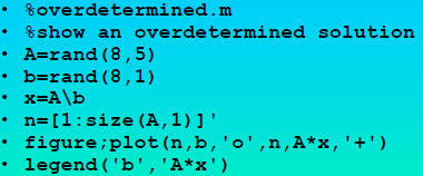
•Over-Determined Systems

–#rows > #columns

•not enough variables for all the equations
–in physics we often deliberately use over-determined systems in
polynomial curve fitting

•reduce the order of the fit to get a smoother curve and to respect the
underlying theory

–for Over-Determined systems with linearly independent rows, a unique
solution can be determined which minimizes the least-squares errors

–we can see this with a very simple code

•Under-Determined Systems
–#rows < #columns
–not enough equations for all the variables
–solution corresponds to an entire subspace: no unique solution
–in physics this is often the sign of an over-excited theorist

•“you can fit any curve with a 7-parameter fit”

•Generally the solution of simultaneous linear equations Ax=b in
physics using MATLAB is obtained with x=A\b

•x=A\b is flexible and intelligent for solving simultaneous linear
equations

•Assuming the rows of A are linearly independent, it will

–for a square system it will seek an exact solution
–for an Over-Determined system it will find a least squares solution
–for an Under-Determined system it will find a solution with the number of
nonzero components less than or equal to the number of equations

•For a square matrix
–a warning message will be issued if the matrix is close to singular
–an error message will be issued if the matrix is singular

Code to Implement Cramer Cramer’s Rule as a Script

Code to Compare Speed of Inversion versus
Gaussian Elimination

Code to Graph Results of an Over Over-Determined
System

More Tutorials

Solution of Simultaneous Linear Equations