
Linear Equations, Inequalities, and Graphs
SQUARING THE VIEWING WINDOW
Section 4.4, Example 9 Determine whether the lines
given by the equations 3x−y = 7 and x+3y = 1 are perpendicular, and
check by graphing.
In the text each equation is solved for y in order to
determine the slopes of the lines. We have y = 3x − 7 and

Since
 we know that the lines are perpendicular. To check this, we graph y1 = 3x − 7
and
we know that the lines are perpendicular. To check this, we graph y1 = 3x − 7
and
 The
The
graphs are shown on the right below in the standard viewing window.
Note that the graphs do not appear to be perpendicular.
This is due to the fact that, in the standard window, the distance
between tick marks on the y-axis is about 1/2 the distance between tick marks on
the x-axis. It is often desirable to choose
window dimensions for which these distances are the same, creating a “square”
window. On the TI-89 any window in which the
ratio of the length of the y-axis to the length of the x-axis is 1/2 will
produce this effect. This can be accomplished by selecting
dimensions for which ymax − ymin = 1/2(xmax − xmin). For example, the windows
[−12, 12,−6, 6] and [−6, 6,−3, 3] are square.
When we change the window dimensions to [−12, 12,−6, 6] and press
 , the graphs now appear to be perpendicular
as shown on the right below. From the equation-editor, Window, or Graph screen,
we could also press
 5 to select ZoomSqr.
When this is done, the calculator will select a square window.
ENTERING AND PLOTTING DATA; LINEAR REGRESSION
We can use the Linear Regression feature on the TI-89 to fit a linear equation to a set of data.
Section 4.5, Example 9 The amount of paper
recovered in the United States for various years is shown in the following
table.
| Years | Amount of Paper Recovered (in millions of tons) |
| 1988 | 26.2 |
| 1990 | 29.1 |
| 1992 | 34.0 |
| 1994 | 39.7 |
| 1996 | 43.1 |
| 1998 | 45.1 |
| 2000 | 49.4 |
(a) Fit a linear function to the data.
(b) Graph the function and use it to estimate the amount of paper that will be recovered in 2003.
(a) First press
 to go to the equation-editor screen and clear any equations that are currently
selected. A check mark
to go to the equation-editor screen and clear any equations that are currently
selected. A check mark
to the left of an equation indicates that it is selected. (See page 125 of this
manual for the procedure for clearing equations.) If
you wish, instead of clearing an equation, you can deselect it. To do this,
position the cursor beside the = sign and press
 .
.
Note that there is no longer a check mark to the left of the equation,
indicating that the equation has been deselected. The graph
of an equation that has been deselected will not appear when
 is pressed. A deselected equation can be selected
again by positioning the cursor beside the = sign and pressing
 . Note that a check mark once again appears to the left of the
equation.
We will enter the coordinates of the ordered pairs in the
Data/Matrix editor. Press
 6 3 to display the new data variable
screen in the Data/Matrix editor. We must now enter a data variable name in the
Variable box on this screen. The name can
contain from 1 to 8 characters and cannot start with a numeral. Some names are
preassigned to other uses on the TI-89. If you
try to use one of these, you will get an error message. Press
 to move the cursor to the Variable box. We will name our
data variable “news.” To enter this name, first lock the alphabetic keys on by
pressing
 .
Then press
.
Then press

 Note that N, E, W, and S are the purple alphabetic operations associated with
the 6,
Note that N, E, W, and S are the purple alphabetic operations associated with
the 6,
 and 3 keys, respectively.
After typing the name of the data variable, unlock the
alphabetic keys by pressing the purple
 key. Now press

 to go to the data-entry screen. Assuming the data variable name “news” has not
previously been used in your calculator,
to go to the data-entry screen. Assuming the data variable name “news” has not
previously been used in your calculator,
this screen will contain empty data lists with row 1, column 1 highlighted. If
entries have previously been made in a data variable
named “news,” they can be cleared by pressing
 .
.
We will enter the first coordinates (x-coordinates) of the
points, as the number of years since 1988, in column c1 and the second
coordinates (y-coordinates), in millions of tons, in c2. To enter the first
x-coordinate, 0 (for 1988), press 0
 .
Continue
.
Continue
typing the x-values 2, 4, 6, 8, 10, and 12, each followed by
 The entries can be followed by
 rather than

if desired. Press
 to move to the top of column c2. Type the y-values 26.2, 29.1, 34.0, 39.7, 43.1,
45.1, and
to move to the top of column c2. Type the y-values 26.2, 29.1, 34.0, 39.7, 43.1,
45.1, and
49.4 in succession, each followed by
 Note that the coordinates of each point must be in the same position in
both lists.
Now use the calculator’s linear regression feature to fit
a linear equation to the data. Press
 to display the Calculate menu.
Press
 5 to select LinReg (linear regression). Then press
 2 to indicate that the data in c1 and
c2 will be used for x and y, respectively. Press
 to indicate that the regression equation should be copied
to the equation-editor screen as y1. Finally press
 again to see the STAT VARS screen which displays the coefficients a
and b of the regression equation y = ax + b. We see that the regression equation
is y = 1.976786x + 26.225.
Note that values for “corr” (the correlation coefficient)
and r2 (the coefficient of determination) will also be displayed. These
numbers indicate how well the regression line fits the data. While it is
possible to suppress these numbers on some graphing
calculators, this cannot be done on the TI-89.
(b) Now we will graph the regression equation. In order to
see the data points along with the graph of the equation we will turn
on and define a plot. To do this, from the STAT VARS screen first press
 to go to the Plot Setup screen. We will
use Plot 1, which is highlighted. If any plot settings are currently entered
beside “Plot 1,”” clear them by pressing
 Clear
Clear
settings shown beside any other plots as well by using
 to highlight each plot in turn and then
pressing
to highlight each plot in turn and then
pressing 
Now we define Plot 1. Use
 to highlight Plot 1 if necessary. Then press
 to
display the Plot Definition screen. The item
to
display the Plot Definition screen. The item
on the first line, Plot Type, is highlighted. We will choose a scatter diagram,
denoted by Scatter, by pressing  1. Now press
 to go to the next line, Mark. Here we select the type of mark or symbol that
will be used to plot the points. We select a box
to go to the next line, Mark. Here we select the type of mark or symbol that
will be used to plot the points. We select a box
by pressing  1. Now we must tell the calculator which columns of the data
variable to use for the x- and y-coordinates of the
1. Now we must tell the calculator which columns of the data
variable to use for the x- and y-coordinates of the
points to be plotted. Press  to move the cursor to the “x” line and enter c1 as
the source of the x-coordinates by pressing
to move the cursor to the “x” line and enter c1 as
the source of the x-coordinates by pressing
 C 1. (C is the purple alphabetic operation associated with the
 key.)
Press
key.)
Press  C 2 to go the the “y” line and
enter c2 as the source of the y-coordinates.
To select the dimensions of the viewing window notice that the years in the
table range from 0 to 12 and the number of millions
of tons of paper ranges from 26.2 to 49.4. We want to select dimensions that
will include all of these values. One good choice is
[0, 15, 0, 60], yscl = 10. Enter these dimensions in the Window screen. Then
press  to see the graph of the
regression line on the same axes as the data.
You can press  if desired, to see the regression equation entered as y1 on
the equation-editor screen.
if desired, to see the regression equation entered as y1 on
the equation-editor screen.
To estimate the amount of paper that will be recovered in 2003, evaluate the
regression equation for x = 15. (2003 is 15 years
after 1988.) Use any of the methods for evaluating a function presented earlier
in this chapter. (See pages 133 and 134.) We will
use the Value feature from the Math menu on the Graph screen.
When x = 15, y ≈ 55.9, so we estimate that there will be about 55.9 million tons of paper recovered in 2003.
THE TRACE FEATURE
Section 4.6, Example 10 Find the domain of f + g if
 and
and 
In the text it is found that the domain of 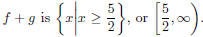 This can be confirmed, at least approximately, by
tracing the graph of f + g. First graph 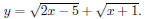 We will use the standard window. Now press
 to select Trace
and use the right and left arrow keys to move the cursor along the curve. We see
that no y-values are given for x-values less than
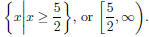
2.5, or
5/2. This indicates that x-values less than 2.5 are not in the domain of f +g. As
we move to the right, ordered pairs appear
to extend without bound confirming that the domain of f + g is